Numerical derivative
Contents
Numerical derivative#
Given a function \(f\), we want to estimate the derivative \(f'\) of \(f\) at a point \(x\) which is not explicitly known.
Introduction#
Derivative are used everywhere. What we’re most interested in is :
Physical systems resolution
Image or signal processing
The numerical derivation will allow us to find an approximation of the derivative using only a discrete set of points, and we will be interested in error estimates.
Functions studied :
Analytical functions (functions for which we know the formula) \(R → R\), continuous and derivable
non-analytical functions but evaluable at any point
a set of points representing a continuous function
I - Derivative calculation#
The derivative of a function \(f(x)\) at \(x = a\) is the limit $\(f'(a) = \lim_{h \to 0}\frac{f(a + h) − f(a)}{h}\)$
We can see that a part of the equation looks like the slope : $\(\frac{f(x_B) − f(x_A)}{x_B − x_A}\)$
If we have the expression of the function, we can derive it by using formal methods of calculation and if we don’t have it, we can estimate it.
The formula above is equivalent to : $\(f_0(x_0) = \lim_{\Delta x \to 0}\frac{f(x_0 + \Delta x) − f(x_0)}{\Delta x}\)$
There are 3 main difference formulas for numerically approximating derivatives.
The forward difference formula with step size \(h\) : $\( f'(a) \approx \frac{f(a + h) − f(a)}{h}\)$
The backward difference formula with step size \(h\) :
The central difference formula with step size \(h\) is the average of the forward and backwards difference formulas :
h can also be represented as \(\Delta x\)
import numpy as np
import matplotlib.pyplot as plt

def derivative(f,a,method='central',h=0.01):
    '''Compute the difference formula for f'(a) with step size h.

    Parameters
    ----------
    f : function
        Vectorized function of one variable
    a : number
        Compute derivative at x = a
    method : string
        Difference formula: 'forward', 'backward' or 'central'
    h : number
        Step size in difference formula

    Returns
    -------
    float
        Difference formula:
            central: f(a+h) - f(a-h))/2h
            forward: f(a+h) - f(a))/h
            backward: f(a) - f(a-h))/h
    '''
    if method == 'central':
        return (f(a + h) - f(a - h))/(2*h)
    elif method == 'forward':
        return (f(a + h) - f(a))/h
    elif method == 'backward':
        return (f(a) - f(a - h))/h
    else:
        raise ValueError("Method must be 'central', 'forward' or 'backward'.")

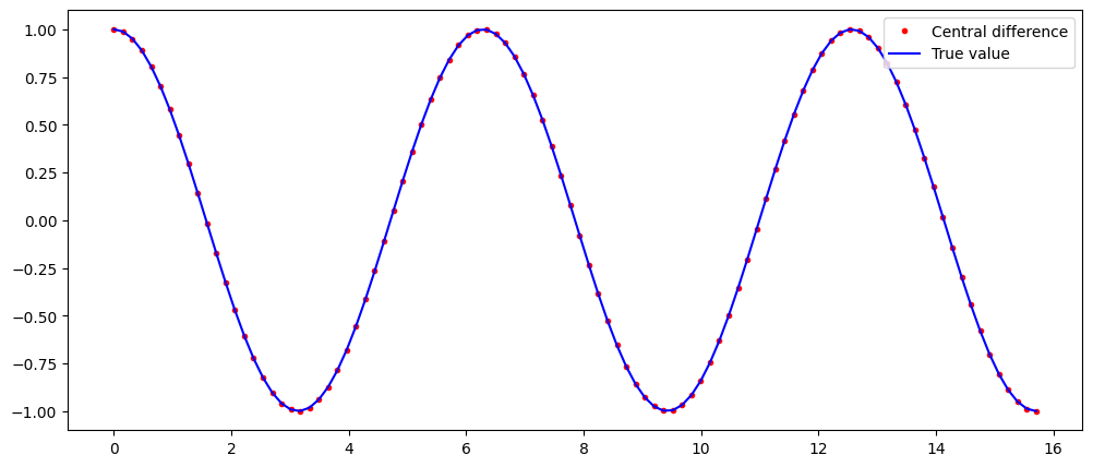
# For example, we can check and plot here the difference between the approximation of the derivative of sinus with
# the central method and the real value
x = np.linspace(0,5*np.pi,100)
dydx = derivative(np.sin,x)
dYdx = np.cos(x)

plt.figure(figsize=(12,5))
plt.plot(x,dydx,'r.',label='Central difference')
plt.plot(x,dYdx,'b',label='True value')

plt.legend(loc='best')
plt.show()

II - Error estimation#
In oder to estimate the error, we need to use Taylor’s theorem.
The degree \(n\) Taylor polynomial of \(f(x)\) at \(x = a\) $\(f(x) = f(a) + f'(a)(x − a) + \frac{f''(a)}{2!}(x − a)^2 + ...\)$
III - Partial derivative#
A Partial Derivative is a derivative where we hold some variables constant.
What about a function of two variables ? (\(x\) and \(y\)):
To find its partial derivative with respect to \(x\) we treat \(y\) as a constant
We know that the derivative of \(x^2\) is \(2x\) We treat \(y\) as a constant, so y^3 is also a constant and the derivative of a constant is 0 To find the partial derivative with respect to y, we treat x as a constant:
We now treat \(x\) as a constant so x^2 is also a constant and the derivative of a constant is 0. The derivative of y^3 is \(3y^2\)
Remember to treat all other variables as if they are constants.

